Excel: 5 timesaving power tips

There’s no such thing as too fast when you’re crunching numbers on deadline in Excel. Any of these power tips will speed up your tasks. Did we miss an even better one? Let us know in the comments. 

1. FORMULATEXT() adds notes to formulas

If you and your colleagues share spreadsheets, it’s nice to have notes that explain what your formulas are doing (plus a copy of the formula). Some organizations even require it, especially if you’re a programmer or analyst.

This little formula and the +N function are the quick answer to your spreadsheet documentation needs. Move your cursor to the column beside the formula column. If that column of cells has additional data in it, you can insert another column (which you can hide when you’re working or printing the spreadsheet), or you can create a separate “FORMULATEXT” matrix out to the side of your original spreadsheet.

The spreadsheet shown below occupies A1 through D15. Move your cursor to E5 and select the FORMULATEXT() function from Formulas > Function Library > Lookup & Reference. In the Reference field of the Function dialog, enter the cell address D5 or just point to it and click OK. Notice that a text version of the actual formula prints in cell E5.

JD Sartain

2. N() function: Another way to add notes

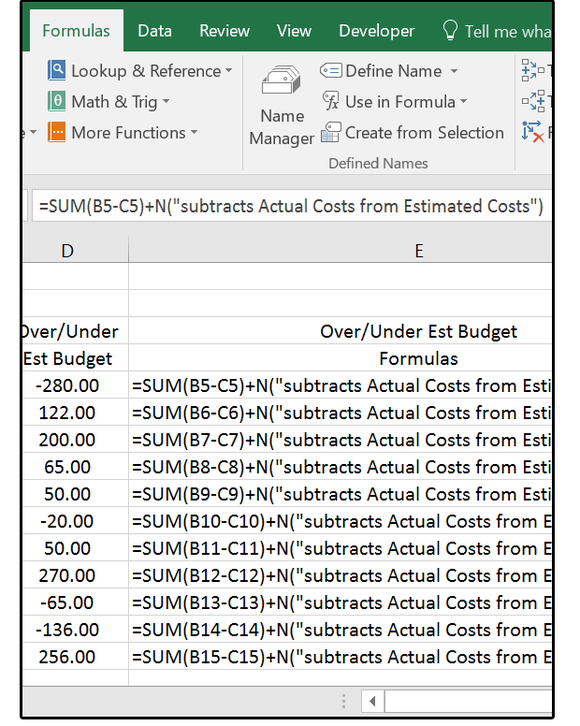
In this example, the formula is self-explanatory, so additional comments aren’t really necessary. However, if this were a long, complicated formula, you could add comments that explain what the formula is doing by just entering +N plus the comment, inside quotes inside parentheses, at the end of your formula in D5. (Note: You would not put it at the end of the Reference in E5.)

For example, move your cursor back to cell D5 and press Function key F2 (to edit your formula). Then type +N(“your comments here”) at the end of your formula (with no spaces). And, if you’d like (although it’s redundant), copy and paste the formula down to D15 and E15.

JD Sartain

3. Case Functions fix upper- and lowercase messes

Have you ever typed an entire paragraph with the caps lock key on? In Word, the solution is an easy shortcut key (Shift+F3 repeated/cycled until the correct case displays). In Excel, it’s a simple function: The UPPER() function converts all characters to uppercase. The LOWER() function converts all characters to lowercase.

Pop quiz: How does one convert upper- or lowercase, or a mixture of both, to what typographers call the Title, Name, or Sentence case? The command in Excel (which is also the preferred term) is Proper case, or PROPER() when written as a function.

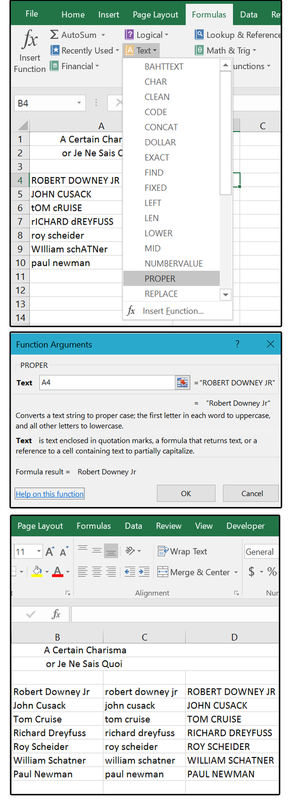
In the sample spreadsheet below, the names are entered in various upper, lower, and proper case formats. Use the Proper function to repair these mistyped names: Move your cursor to cell B4, then click Formulas > Function Library > Text. From the Text dropdown, select Proper.

The Function Arguments dialog box will appear. In the Text field, enter or point to cell A4, then click OK. Copy B4 down through B10 and notice how the Proper function has repaired all the mistyped names in this list.

Next move your cursor to cell C4 and enter the Lower function, which you can find in the same Text dropdown menu or enter it manually in cell C4: =LOWER(B4) and press Enter.

Move your cursor to D4 and enter the Upper function in this cell, or write =UPPER(B4) and press Enter. Copy cells C4 and D4 down thru C15 and D15. Now each name in each list is displayed correctly. Note that these functions also work for imported or copied text.

JD Sartain

03 Use the Case functions UPPER(), LOWER(), AND PROPER() to repair case typing errors

4. Transpose feature to rearrange columns and rows

All super users know that in Excel fields are placed in columns and records are placed in rows. However, sometimes you inherit a spreadsheet from a rookie who has it backward. Retyping all that data is out of the question, and using copy/paste one row at a time would be horribly tedious. This doesn’t seem like a big deal on a small spreadsheet, but imagine reorganizing 40 columns and 200 rows and you’ll like this tip much better.

Highlight the data matrix you want to transpose (in our example, it’s A1 through F6). Select Copy. Move your cursor to the new, target location. Go to Home > Clipboard and click Paste > Paste Special. In the Paste Special dialog box, check the Transpose field box, and click OK. And that’s it! The data moves to the new location with the columns and rows transposed.

JD Sartain

5. Save more seconds with Autofill

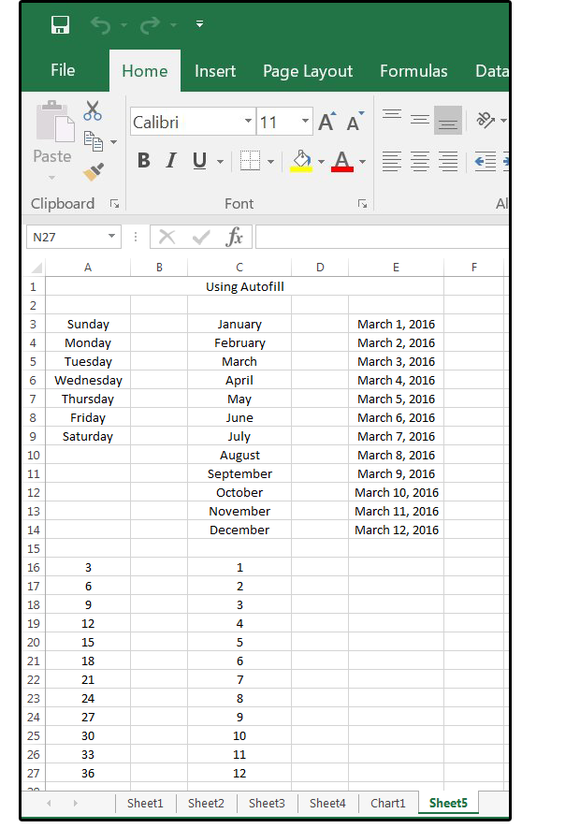
Everyone who handles series data should use Autofill to save typing and retyping for things that are always the same—for example, a list of consecutive numbers or letters, months of the year, or days of the week.

1. Enter a day of the week in cell A3.

2. Hover the cursor over the bottom right corner of the cell until it changes to a black cross.

3. Click and drag horizontally or vertically to copy the content down or over.

Notice the tag following your cursor as it drags. The info inside the tag changes to the next item in the series (in this case, the next day of the week).

JD Sartain

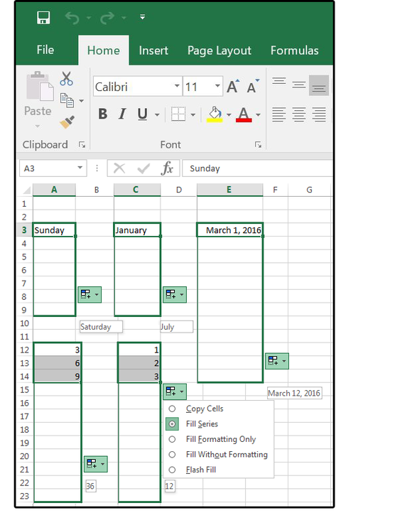
4. When you release the left mouse button, the Autofill Options icon appears (overwriting the black cross). Click the down arrow and note the options available:

Copy CellsFill SeriesFill Formatting OnlyFill Without FormattingFlash Fill

If not already selected, click the Fill Series button.

The series displays (in consecutive order) up to the point where you stopped dragging the cursor.

JD Sartain

Note: If the Autofill Options icon does not appear when you stop dragging the black cross, Select File > Options > Advanced. Scroll down to the Cut, Copy, & Paste section. 

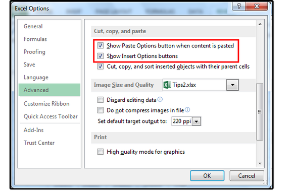JD Sartain

You’ll see these three options with radio buttons:

Show Paste Options button when content is pastedShow Insert Options buttonsCut, copy, and sort inserted objects with their parent cells

Ensure that the first and second buttons are both clicked on. (The third button is optional.)