Excel tips: 6 slick shortcuts, handy functions and random-number generators

Simpler and faster is always better in Excel. We start with some of my favorite shortcuts, then move on to using Excel for everyday situations such as finding random numbers for passwords, or random numbers within a range, or discovering how much your monthly payments will be for a car or home loan.

1. Shortcut: Select the entire spreadsheet

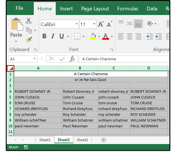
Everyone knows that Ctrl+A selects the entire spreadsheet, document, email, etc. In Excel; however, there’s an even faster way: Click the small green arrow in the square space between the row numbers and column letters.

JD SARTAIN

2. Shortcut: Number formats

Which is faster—the mouse or the keyboard? Those who use both work faster than either one or the other alone. Try these shortcuts: After you enter a number or column of numbers, highlight the target cells and press…

Ctrl+Shift+! (exclamation point) to display the Number format with two decimal points,

Ctrl+Shift+$ (dollar sign) to format the selected cells as currency,

Ctrl+Shift+% (percent sign) to format as percentages,

Ctrl+Shift+~ (tilde) for the General format,

Ctrl+Shift+# (pound sign) for the Date format,

Ctrl+Shift+@ (at sign) for the Time format, and

Ctrl+Shift+^ (caret) for the Exponential number format.

JD SARTAIN

3. Shortcut: Quick Zoom

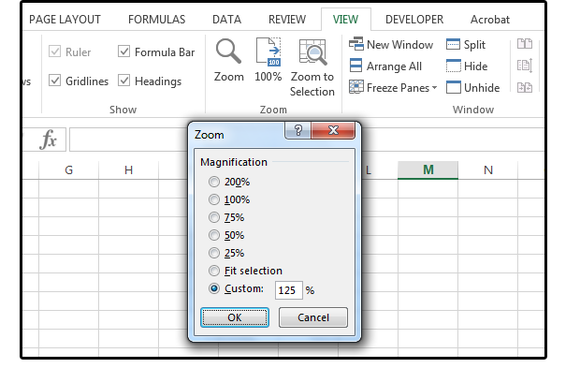
If you want to zoom in or out of your spreadsheet, you have to perform several steps: First select the View tab, then select the Zoom button in the Zoom group, then select a Zoom Magnification from the Zoom dialog box (or click Custom and type a Zoom Magnification size in the field box), then click OK. Whew!

How about this simple shortcut instead: Hold down the Ctrl key and roll the mouse’s scroll wheel forward to zoom in or backward to zoom out. Easy.

Note: This shortcut also works in Word, Outlook, PowerPoint, Windows, and the Internet (i.e., Internet Explorer, Chrome, Mozilla Firefox, etc.).

JD SARTAIN

4. The PMT function

Ever wonder how much your house or car payment would be for a specified loan amount? Imagine having the tools to determine if you can afford a Prius or a Camry; a house or a condo? Say, for example, the house cost $200,000 for a 30-year loan at 3.2% interest? Use the PMT formula to find out. In cell A3, enter this formula: =PMT(3.2%/12,360,200000).

Note the answer is ($864.93). Why is it displayed as a negative number? Because it represents money that you pay out (as opposed to money you receive).

Now, instead of piling all the information into a single formula, place the data into separate cells so you can change the numbers and play around with the payment amounts. For example, enter the following field names in columns A, B, C, D, and E: Interest Rate, Divide by Months In the Loan Year, Term (in Months), Loan Amount, and Payment.

Now enter some data into these fields; for example: in A7 enter the current market interest rate. Next (in B7), if the rate is per year (which is almost always), enter 12 (for 12 months in the year. In column C, enter the term or length of the loan (in months, not years). Last, enter the loan amount in D7.Then enter this formula in the Payment field (E7): =PMT(A7/B7,C7,D7). The answer is ($1100.65).

Now you can change the values in A7 through D7 (or copy the information down) and enter different interest rates, loan amounts, and terms to find out how much the payments are for your next house, car, boat, or any other loan.

JD Sartain

5. The RAND function

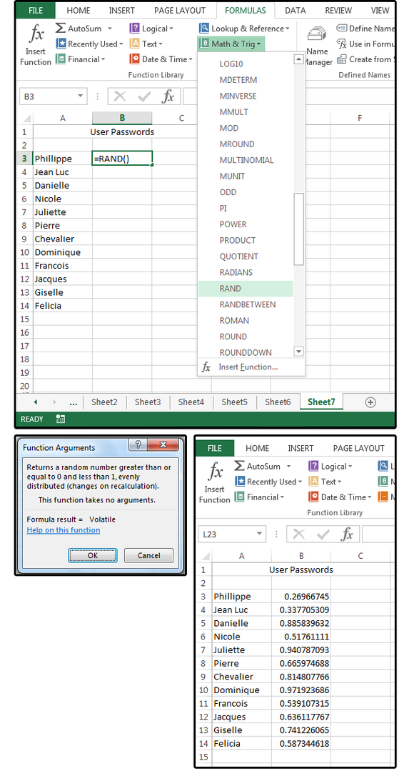
If you’re one of those disciplined few who changes your password every week or month, or you manage the passwords of users on a network; the RAND function is your best friend because the numbers really are random. You can create a list in Excel, use this function to create the passwords, then pass them out to your staff. And because Excel recalculates formulas every time you press the Enter key and every time you save and exit, the numbers will never be saved anywhere.

NOTE: RAND numbers are between 0 and 1. You can remove the preceding decimal for your passwords.

Enter 12 names in cells A3 through A14. Move your cursor to cell B3. Go to Formulas > Function Library > Math & Trig, and select the RAND function from the dropdown menu. Note the dialog box says “This function takes no arguments.” That means you don’t have to do anything except click OK. Copy the function from B3 down to B14. Notice that every time you press Enter, the numbers change.

JD Sartain

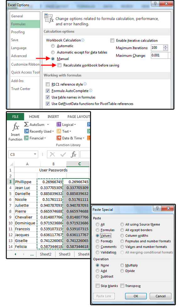
To keep a record of the random numbers, use the VALUE() command or Copy > Paste > Paste Values to create a static list of the numbers in column B. However, you must first turn off the Auto Calculation (set it to Manual), or the random numbers/passwords will change the second you press Enter.

To change Auto-Calc to Manual, select File > Options > Formulas. At the top of the screen under Calculate Options, check Manual and uncheck Recalculate Workbook Before Saving. Now you can copy the random numbers/passwords in column A to column B. Highlight A3 through A14. Type Ctrl+C for Copy. Move to B3 and select Paste Special from the Home tab’s Clipboard group. Then check Values in the Paste Special dialog box and click OK. Now you have a copy of the random numbers in column A.

JD Sartain

Press F9 to recalculate the spreadsheet while in Manual Calc mode, or you can change the Manual Calc back to Auto Calc.

Note: The Option settings are based on the spreadsheets that are open at the time. In other words, if you open a Manual Calc spreadsheet first, the Options will still be set to Manual Calc. Any other spreadsheets you open (at the same time) will also be set to Manual Calc. But if you open a new, blank spreadsheet (or another Auto Calc spreadsheet) first, where the default Auto Calc is set in the Options, all other spreadsheets you open simultaneously (even this one) will be set to Auto Calc.

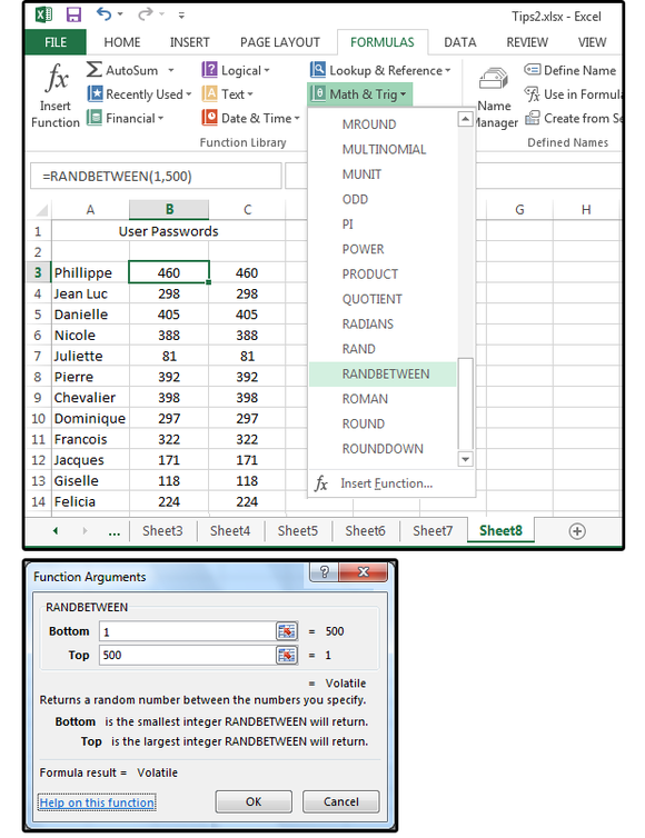
6. The RANDBETWEEN function

The RANDBETWEEN function is just like the RAND function, except you get to choose the range of numbers—for example, between 1 and 500, or 10 and 1,000. Once you remove the decimals in the RAND command, the random numbers created are good for most all situations. But if you specifically want four-digit or six-digit numbers only, use RANDBETWEEN and choose a range of numbers that fall into that requirement.

NOTE: The same rules apply for Manual Calc and using Copy > Paste > Paste Values to make a copy of the random numbers before they change again.

Use the same names as in the previous spreadsheet (on cells A3 through A14). In cell B3, select the RANDBETWEEN function from Formulas > Function Library > Math & Trig. In the Function Arguments dialog box, enter the bottom (lowest) number of your range and a top (highest) number of your range, then click OK. Copy the formula from B3 down through B14, then press F9 so the formula calculates. Then move to C3 and Copy > Paste > Paste Values.

JD Sartain